Chapter 16: Networks

In this module, we’ll look at D3’s approach for building network visualizations. While there are many ways of visualizing networks (adjacency matrices, hive plots, dendrograms, etc.), this module focuses on methods for explicitly visualizing network graphs.

If you prefer watching entertaining videos to reading tutorials, I suggest you watch this talk by Jim Vallandingham, which captures and explains these ideas incredibly well.

Helpful links:

• Force Layout (D3 Wiki)
• Abusing the Force (Vallandingham, OVC Video)
• Bostock Explains Networks (Bostock, Meetup Video)
• Bostock Explains Networks (Bostock, Meetup Video Slides)

16.1 Network Data

Before we talk about visualizing network data, we should briefly discuss the structure of network data. Network data captures information regarding a set of elements and the relationships between them. To use network vocabulary, we’ll use the following terms:

Elements: each element or observation in your dataset is represented as a symbol in your graph, frequently referred to as a node or a vertex. These symbols often appear as symbols, but may be text, images, or other representations.

Relationships: Network data captures information about the relationships (or connections between) elements. Ties between elements may be directionless (i.e., two friends share a mutual connection) or directed (i.e., payment flowed from a source node to a target node). Relationships are commonly depicted as lines (paths) between nodes, and referred to as links or edges.

Below is a simple dataset that captures relationships between elements, and an example of how that data could be represented in a graph. Open up demo-1 to interactively edit the underlying dataset (note, the implementation is imperfect).

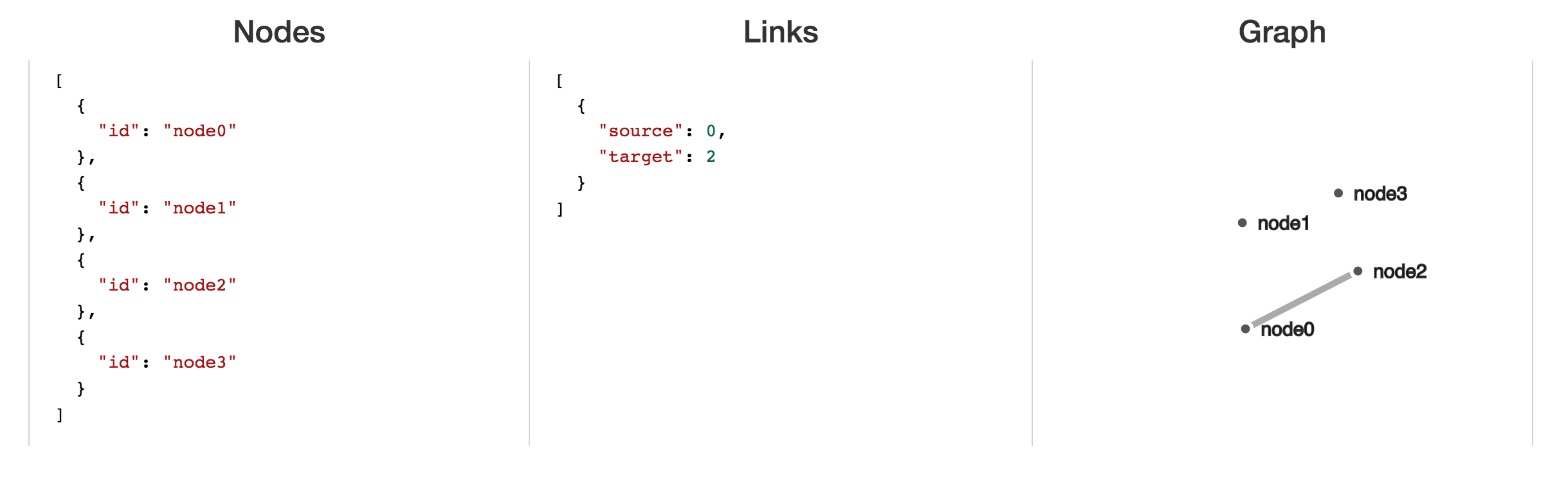
screenshot of node and link data with graph

16.2 Force-Directed Layout Overview

In order to understand the methods below, you must first understand what is actually happening when D3 builds a network visualization. Unlike other layouts in which we have explicit position for underlying data values, network visualizations do not have a single solution for expressing the elements in the dataset and all of their connections. Building a network visualization is an attempt to meet certain aesthetic constraints in a rendering area, such as:

• Minimize edge crossings
• Maximize layout symmetry
• Minimize edge length variance
• Minimize longest edge
• Minimize bends towards straight lines

A common approach for computing a layout that meets these constraints is to leverage a physical simulation that facilitates the optimization of given requirements. The layout we’ll describe is the force-directed layout, which applies the following behaviors in order to achieve the constraints:

Nodes act as charged particles that repulse and attract one another.

Edges act as geometric constraints that determine the distance between nodes

Through iterative physical simulation, the optimal layout of nodes is computed. In each step of the simulation, the positions of the nodes are adjusted according to a variety of physical forces (attractions / repulsions) until a threshold level of constraints is met. The important takeaway for this learning module is that node positions are updated repeatedly until the simulation converges.

16.3 Force Layout Simulation

Similar to other layouts, D3 provides a method for computing force directed layouts with the d3.layout.force method. Not surprisingly, this is a function that returns a function, enabling you to specify a variety of behaviors about the simulation forces necessary to compute the layout. Here are some of the parameters you will want to adjust to manipulate your layout:

• nodes: An array of objects specifying the vertices you want to represent.
• links: An array of objects specifying the edges you want to represent. Even if your data is undirected, you’ll use the terms source and target the specify the node indices that should be connected.
• size: An array indicating the width and height of the plotting area.
• friction: This parameter (suggested to be in the 0 - 1 range) specifies the rate at which the velocity of each node will decline at each step in the simulation.
• gravity: A numeric value that sets a weak geometric constraint on the simulation by applying a spring-like force between each node and the center of the layout. This prevents nodes from escaping the layout.
• linkDistance: Sets the target link distance for the layout. Link distances in the simulation are compared to target distances. Defaults to -30.

• charge: A numeric value specifying the repulsion of each node. Defaults to -30.

• linkStrength: A value in the range 0 - 1 specifying the rigidity of the links .

Here is an example of declaring a force function:

// Set force function
var force = d3.layout.force()
    .gravity(.05)
    .distance(100) // Desired distance
    .charge(-100) // Negative number indicates repulsion
    .size([width, height]) // Set width and height
    .nodes(nodes) // Pass in elements as `nodes`
    .links(links); // Pass in edges as `links`

Note, while many of these parameters accept single values, they also accept functions, allowing you to use data values of your links or nodes to drive the layout of the graph (most notably linkDistance and charge). For full descriptions of each parameter, see the documentation. While the code snipit above specifies the behavior of your simulation, it does not initiate it. Not surprisingly, you use the .start() method to initialize your simulation, which will compute your layout on the specified nodes and links.

Importantly, passing your node data to your force function changes your data. The following attributes are computed using the nodes function (from documentation):

• index - the zero-based index of the node within the nodes array.
• x - the x-coordinate of the current node position.
• y - the y-coordinate of the current node position.
• px - the x-coordinate of the previous node position.
• py - the y-coordinate of the previous node position.
• fixed - a boolean indicating whether node position is locked.
• weight - the node weight; the number of associated links.

16.4 Implementing the Force Layout

As noted above, the .start method initializes your simulation, iteratively re-positioning elements to find an optimal layout that satisfied the specified restraints. Each step in the simulation is registered as a tick event. In order to visually represent the progress of the simulation, you’ll want to specify an event-handler that changes element position each time the tick event occurs. For example:

// Select all elements with class link to perform a data-join
var link = svg.selectAll(".link")
              .data(links)

// Select all elements with class node to perform a data-join
var node = svg.selectAll(".node")
               .data(nodes, function(d) {return d.id;})

// Enter/append symbols for links (lines) and nodes (circles)
...

// On tick function for each step in the simulation
force.on("tick", function() {
  // Reset attributes for each line
  link.attr("x1", function(d) { return d.source.x; })
      .attr("y1", function(d) { return d.source.y; })
      .attr("x2", function(d) { return d.target.x; })
      .attr("y2", function(d) { return d.target.y; });

  // Reset the transform/translate property for each circle element
  node.attr("transform", function(d) { return "translate(" + d.x + "," + d.y + ")"; });
});

In order to begin computing your layout (and assigning the associated x and y properties to each piece of data), you’ll need to initialize the simulation using the .start method:

force.start() // initialize the simulation